Intact Tombs Analysis
Data Science · K-Means Clustering, Jupyter, Statistical Testing, Data Analysis
Abstract
This study analyzes intact and nearly intact New Kingdom tombs from Thebes to assess whether burial assemblages can be placed into well-defined groupings based on the socioeconomic statuses of those within them. Building on Smith’s (1992) “manually” established tomb groupings, we employ several multivariate statistical approaches, including PERMANOVA, PERMDISP, pairwise distance analysis, and K-Means clustering, to evaluate the consistency and distinctiveness of these groupings. While PERMANOVA suggests significant group differences, PERMDISP reveals high variance in group dispersions, debunking those results. Pairwise distance analysis supports Smith’s classifications, showing lower within-group variability and higher between-group differences. In contrast, the K-Means algorithm produces alternative clusters driven less by total tomb valuation and social dynamics and more by the specific composition of burial goods, identifying distinct provisioning patterns related to fertility items, furniture, and vessels. Together, these approaches offer complementary perspectives on both systemic and individualized aspects of funerary behavior in the New Kingdom.
Analysis of Manual Groups from Smith (1992)
Smith (1992) classifies 134 tombs into five socioeconomic groups based on the quantity, quality, and types of grave goods, ranging from Tutankhamen as uniquely lavish, through elite/high-middle/middle categories, to a broad low-status group. To test whether these groupings have statistical support, MANOVA was avoided because the data are skewed and group sizes are highly unbalanced, so we used PERMANOVA (Euclidean distance) to test centroid differences in multivariate space; it indicated significant differences among groups (p = 0.001). However, because PERMANOVA can be confounded by unequal within-group spread, we ran PERMDISP, which showed extreme dispersion differences across groups (p = 2.2e-16), weakening confidence that the PERMANOVA result reflects centroid separation alone.
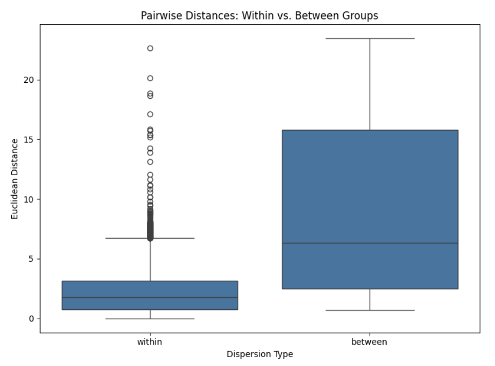
Given this, we examined pairwise distances to compare within-group versus between-group variability directly. On average, between-group dispersion was higher than within-group dispersion, suggesting the categories still capture meaningful overall separation, but several strong within-group outliers were identified. The largest contributors were S+ (96 outlier-distance instances), Nu+ (91), and DeM 1381 (85), with most other tombs contributing fewer than 18; notably, all three belong to the low-status group and are relatively high spenders within it, which likely drives their outlier behavior.
K-Means Clustering
It is also valuable to explore inherent groupings of the tombs that emerge from the natural structures present in the data. In this way, we can attempt to discover which tombs are more similar to each other based solely on their quantitative characteristics. To do this, we use the K-Means clustering algorithm. We set K = 5 to follow along with the original groupings established by Smith (1992) - Tutankhamen, Elite, High-Middle, Middle, and Low Status. This is partially to test whether the algorithmically determined clusters will align with the manual groups. The tombs were assigned as follows:
| Cluster 0 | Cluster 1 | Cluster 2 | Cluster 3 | Cluster 4 |
|---|---|---|---|---|
| All Other Tombs | Tutankhamen | Y&T (Yuya and Tuya) | Mahirper | K&M (Kha and Merit) |
| Setau | M+ | Hatnofer | ||
| DeM 1381 | S&N (Sennofer and Nefertiti) | |||
| DeM 1389 | ||||
| DeM 1375 | ||||
| Neferkhewet | ||||
| I+ | ||||
| SR+ |
Out of the 134 tombs in this analysis, 120 of them are assigned to Cluster 0. All of these tombs had a grand total cost of less than 565 db, and therefore nearly all of these tombs would be considered to be of Low Status according to the typology established in Smith (1992). For the full list of tombs in Cluster 0, please see Appendix A. Cluster 1 is occupied by only King Tutankhamen. Given the extraordinarily high cost of Tutankhamen’s burial, it is unsurprising that the algorithm isolates him into a cluster of his own, mirroring the distinction made in the original classification. It is in Cluster 2, Cluster 3, and Cluster 4 that we see major deviations from the original groupings. None of these clusters seem to reflect the socioeconomic differences that are highlighted by Smith (1992), and in fact have highly variable tomb valuations. We evaluate each of these three clusters in turn.
Cluster Interpretation
Tutankhamen’s tomb stands apart because his overall spending is so extreme that it effectively places him in a cluster by himself. Similarly, the majority of the other tombs were extremely low cost and it is likely that these were all grouped together into cluster 0 for this reason. For the remaining clusters, several tombs can look “misplaced” when considering total expenditure, but looking at how each cluster’s spending is distributed across provisioning categories helps explain why they were grouped together despite large differences in overall worth. Our analysis suggests that the clustering reflects not just how much was spent, but what it was spent on. Categories like fertility products (items associated with regeneration and rebirth) and vessels (containers for food, drink, and offerings) could make up meaningful portions of a tomb’s budget and differentiate burials with similar priorities.
Cluster 2 pairs Setau with Yuya and Tuya even though Yuya and Tuya’s tomb is far more valuable, because both share an unusual pattern of very high fertility provisioning (the highest in the dataset) alongside minimal or zero spending in several other categories. Cluster 3 also mixes high and low cost tombs, but the link is more specific: the high-spending tombs in this cluster are unusual precisely because they have little or no furniture, which separates them from other elite burials where furniture is a major expense. Meanwhile, the lower-cost tombs in Cluster 3 are unusual in the opposite direction, consistently including some furniture and spending more on it than typical low-status burials in Cluster 0. This combined with a notable consistency across several other provisioning categories including fertility products, toiletries, boxes and baskets, bouquets, and vessels may have contributed to the fomration of this cluster. Cluster 4 is best explained by vessels as a share of total value, with tombs in this group devoting far larger proportions of their budgets to vessels than any other cluster; even the lower-valued Sennofer and Nefertiti tomb stands out on this measure, linking it to the other tombs in the cluster. To see my extensive analysis with the accompanying figures, please take a look at the full report available on the Github linked at the top of this page.
Visualizing The Tombs in PCA Reduced Space
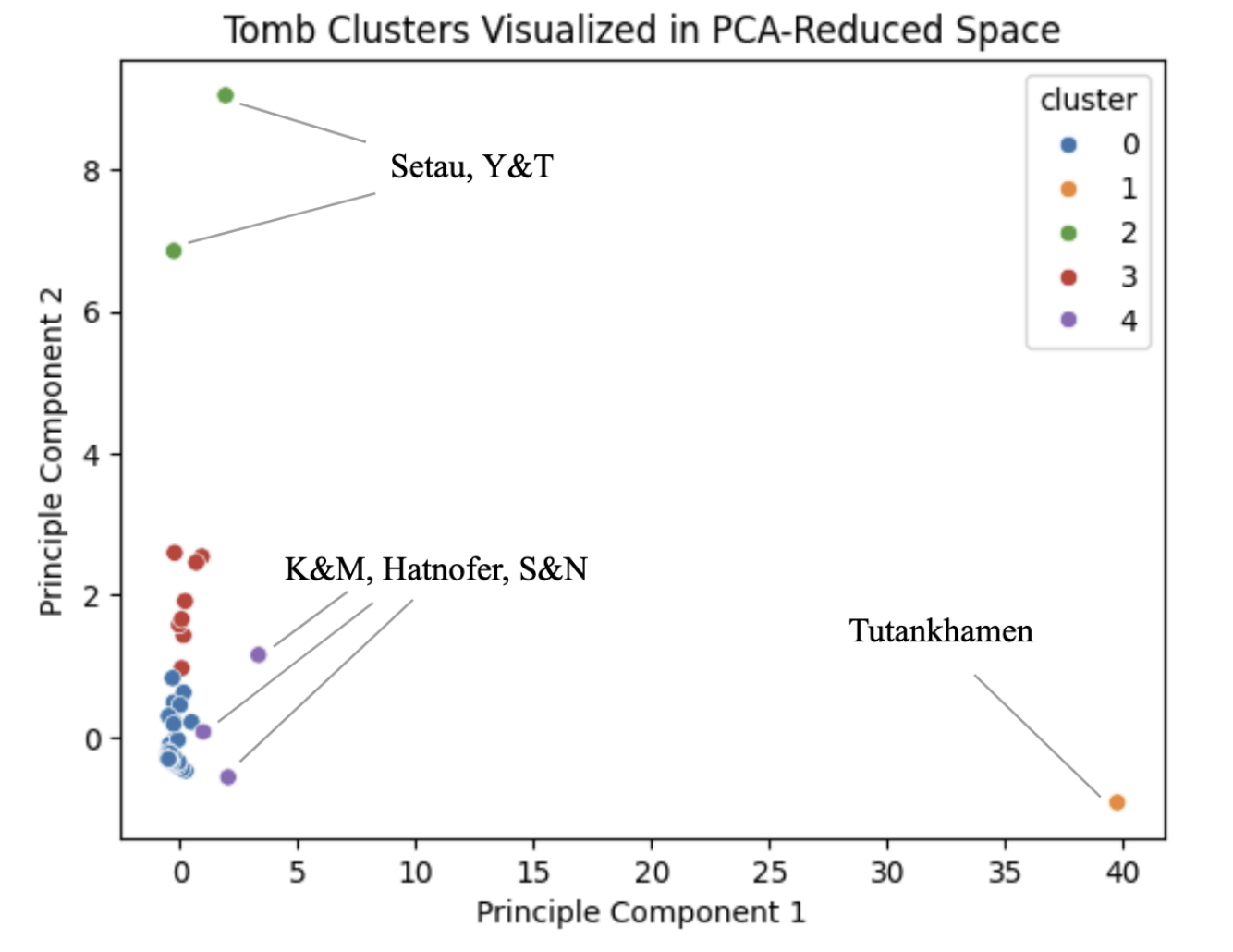
Plotting all five clusters in the PCA-reduced space can help visualize the structure and separation of the groups. The placement of Tutankhamen far along Principal Component 1, and Setau along with Yuya and Tuya high on Principal Component 2, provides some insight into what these principal components may be capturing. Principal Component 1 may largely reflect overall tomb valuation, given Tutankhamen’s exceptionally high total cost, while Principal Component 2 may be influenced by fertility spending, as Setau and Yuya and Tuya are the highest spenders in this category. However, it is important to note that PCA creates linear combinations of all input features, and each principal component may reflect contributions from multiple factors simultaneously. While tomb valuation and fertility spending appear to be important drivers, other provisioning categories likely contribute as well, and the true interpretation of these components remains approximate. Nonetheless, this separation helps illustrate how varying provisioning patterns across different categories can contribute to the formation of distinct clusters.
Learnings & Takeaways
- End-to-end statistical design: This project taught me how to design and execute a complete statistical analysis, from defining research questions that are both answerable with available evidence and meaningful for the broader argument, to selecting appropriate methods and justifying analytical choices.
- Interdisciplinary collaboration and ownership: Working with an expert in a field far from my own required me to take full ownership of the quantitative side. I had to arrive with a plan, explain how each step connected to research goals, and defend decisions about feature construction, normalization, clustering choices, and interpretation.
- Translating technical outputs to domain insights: I learned to translate statistical outputs into domain-relevant claims and explain why those claims were warranted, bridging the gap between quantitative methods and archaeological argument.
- Rigorous data preparation: Understanding and preparing the archaeological dataset was the biggest challenge. Many variables reflected unfamiliar artifact typologies and provisioning categories, and the raw data contained inconsistencies requiring substantial background reading and extensive data cleaning.
- Quality inference depends on data handling: Standardizing labels, resolving missing entries, verifying totals, and restructuring data for statistical modeling ultimately shaped the analysis quality, reinforcing that rigorous inference depends fundamentally on careful, well-justified data handling.