Regularization and Its Effects on Spurious Feature Learning

Abstract

Modern neural networks often achieve high accuracy by relying on spurious features: shortcuts that correlate with the label in training but fail to generalize. While prior work has shown that core features are still learned even when spurious shortcuts are present, less is understood about how regularization reshapes the internal trajectory of feature emergence across depth and training time. Using linear probes attached at six depths of a ResNet-18, we study how L1, L2, and dropout regularization alter where and when spurious versus core features become linearly accessible. Using Colored MNIST and Waterbirds as controlled testbeds, we find that each method of regularization reshapes the depth-wise trajectory differently. Moderate regularization restricts spurious feature propagation into deeper layers without harming core feature learning, while aggressive regularization destabilizes both.

Background

Deep neural networks perform very well on many tasks, but they often rely on spurious features—patterns in the data that are correlated with the label but are not actually meaningful. For example, a model might use the background color of an image instead of the object itself to make predictions. This leads to poor performance when the data distribution changes, especially for rare or minority cases.

Previous work by Izmailov et al. (2022) shows that even when models rely on these shortcuts, they may still learn the correct core features internally. The main difference is how these features are used in the final layer. However, this work only looks at the final trained model and does not explain how these features develop during training or where they appear inside the network.

We ask: when does the model first learn the spurious feature? When does it learn the core feature? And at what point does the core feature become more important than the spurious one? We study whether regularization delays or reduces the learning of spurious features and helps the model focus more on core features, tracking these dynamics across both layer depth and training time.

Methods

We train ResNet-18 models on two controlled datasets. Colored MNIST is a binary classification task (digits 0–4 vs. 5–9) where each image is colored red or green with 90% correlation to the label, making color a learnable shortcut. Waterbirds places bird images onto water or land backgrounds with 95% correlation, making background the spurious feature.

To measure how much information about each feature is present at different depths of the network, we attach linear probes at six points in the ResNet-18: the initial ReLU, the outputs of layer1 through layer4, and the global average pool. A linear probe is a single linear classifier trained on the frozen activations of a given layer. If a probe achieves high accuracy on a particular feature, that feature is linearly accessible in that layer's representation. By training separate probes for the core feature (digit class or bird type) and the spurious feature (color or background), we can track where and when the network encodes each one during training.

We test three regularization methods at varying strengths: L1 regularization (λ = 1e-5, 1e-3, 1e-2), L2 regularization (λ = 1e-5, 1e-3, 0.1), and Dropout (p = 0.1, 0.3, 0.5). Results are visualized as heatmaps where the x-axis represents training epoch, the y-axis represents layer depth, and cell color indicates probe accuracy from red (low, ~0.5) to green (high, ~1.0).

Baseline Behavior

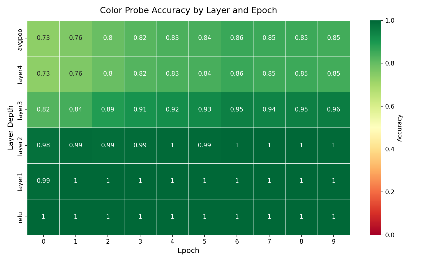
Color (spurious) probe accuracy

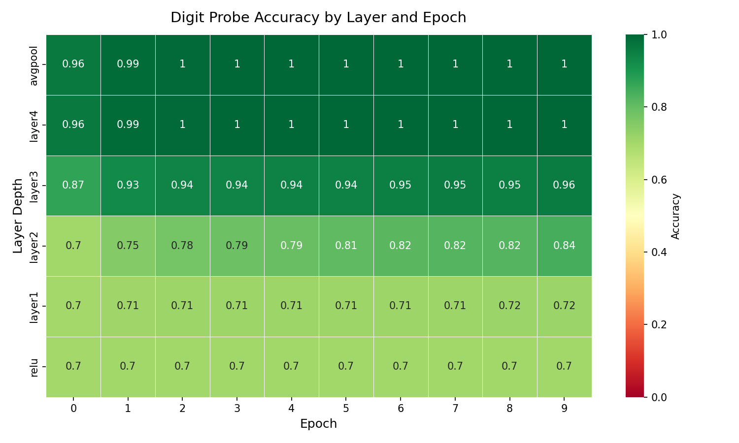
Digit (core) probe accuracy

Without any regularization, the model learns both features quickly. Color probe accuracy saturates in the early layers within the first epoch and remains high throughout training. Over time, color also becomes increasingly readable in the deeper layers, spreading from the early layers into layer3, layer4, and avgpool. Digit probe accuracy builds progressively with depth, reaching near-perfect accuracy in the later layers. The model achieves 99.29% accuracy. This baseline establishes the default behavior: early and persistent encoding of the spurious feature, with gradual spread into deeper layers over training.

How Regularization Reshapes Feature Trajectories

Our central finding is that regularization does not simply suppress spurious features uniformly—each method reshapes the depth-wise trajectory in a qualitatively different way.

L1 Regularization

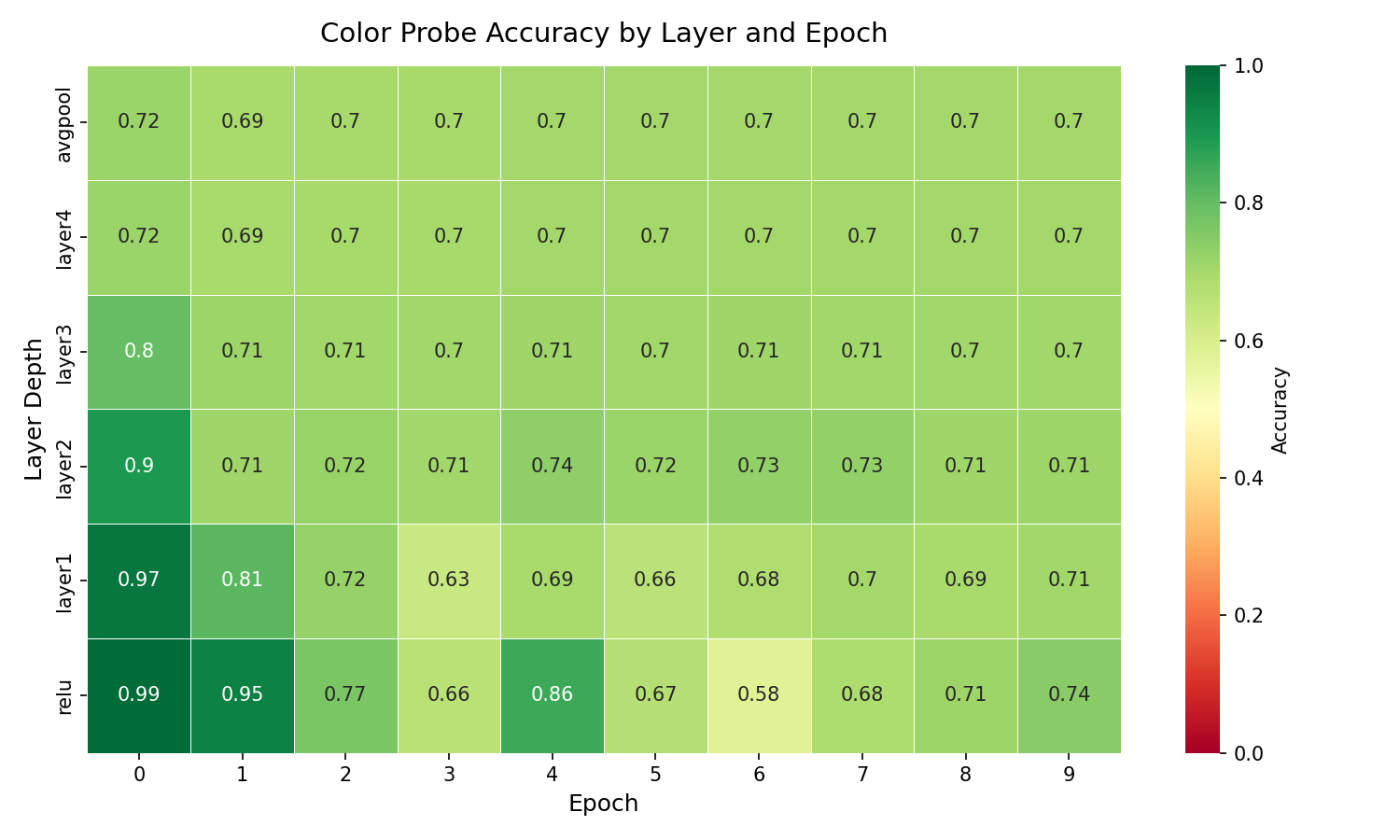
Color (spurious) probe accuracy

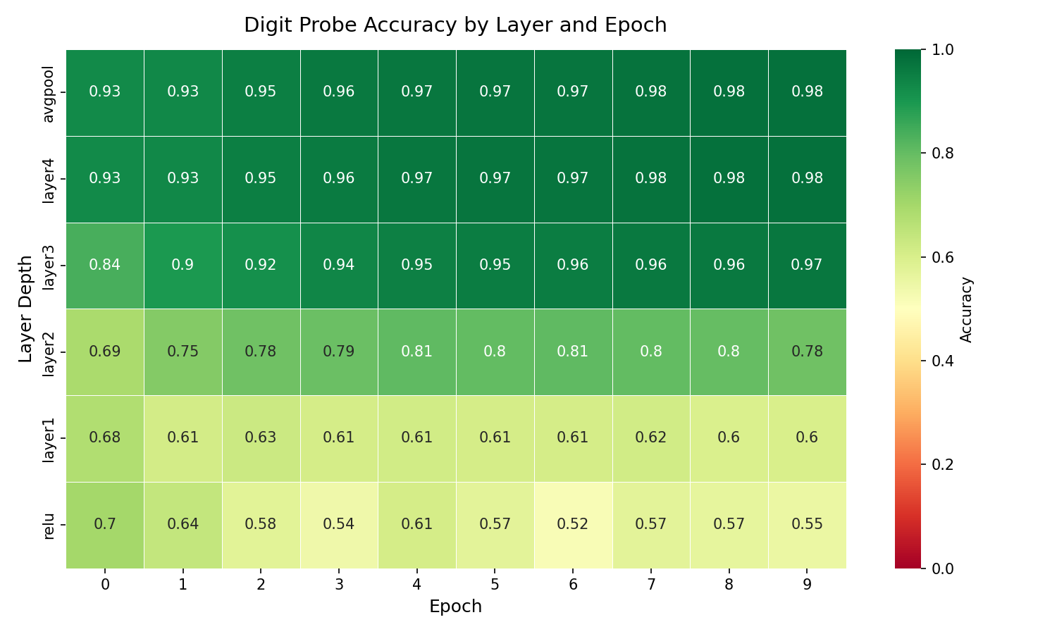
Digit (core) probe accuracy

At moderate strength (λ = 1e-3), L1 achieves the best trade-off. Color features are still learned early but are less dominant than in the baseline. Early layers (ReLU, layer1) initially show high color probe accuracy (0.99, 0.97), but this decays over training epochs rather than spreading into deeper layers. Digit features improve steadily with depth, reaching 0.98 in the later layers by the final epoch. The model achieves 97.79% accuracy with 98.35% precision and 97.08% recall. Increasing L1 strength constrains feature learning across all layers uniformly—unlike L2, which selectively blocks deeper layers, L1's sparsity pressure suppresses features more broadly.

L2 Regularization

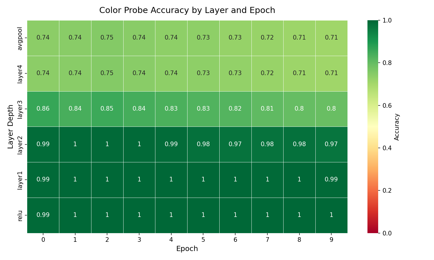
Color (spurious) probe accuracy

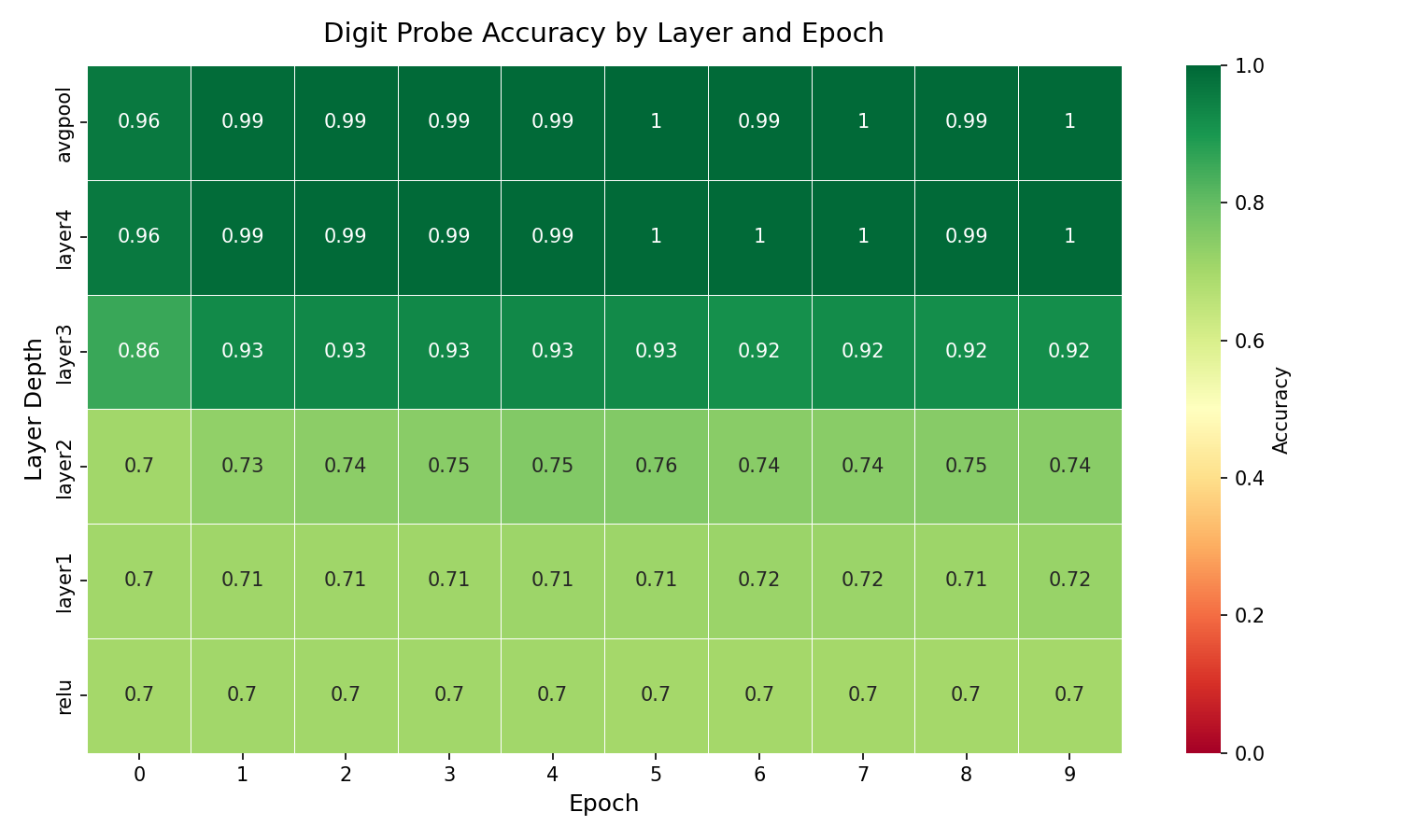
Digit (core) probe accuracy

At moderate strength (λ = 1e-3), L2 selectively prevents spurious features from leaking into deeper layers. Color is encoded in the early layers (ReLU through layer2) but does not spread into the deeper layers over the course of training. It remains fixed in the early layers throughout. Digit shape is well-preserved in deeper layers (layer3, layer4, avgpool). The model achieves 99.20% accuracy. This selective blocking—constraining the spread of spurious representations without suppressing them entirely—distinguishes L2 from L1's more uniform pressure.

Dropout

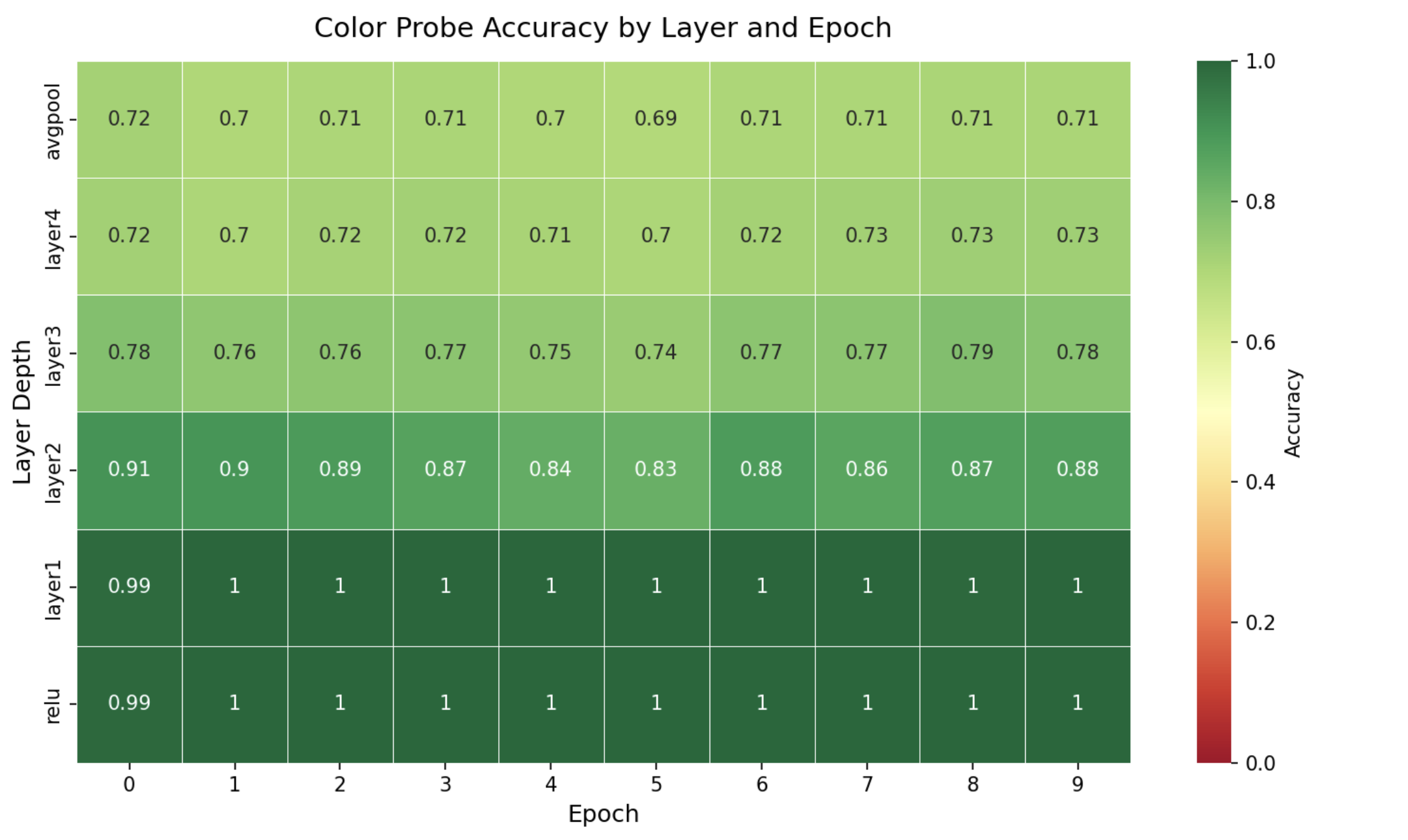
Color (spurious) probe accuracy

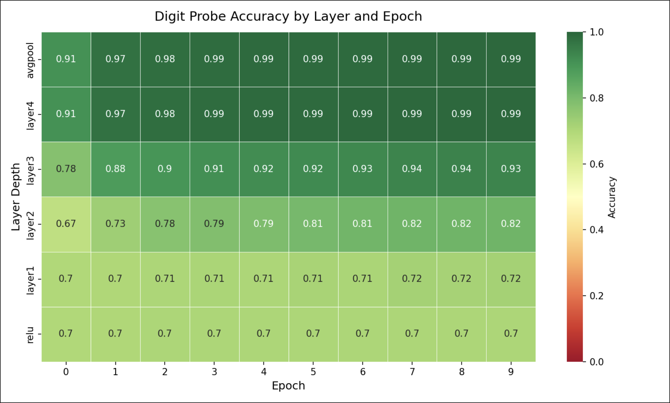
Digit (core) probe accuracy

At p = 0.5, dropout produces the strongest suppression of spurious feature propagation. Color still saturates in the very early layers (the initial encoding is unaffected), but color accuracy in layer2 actually decreases over training, suggesting active suppression of spurious feature propagation rather than passive prevention. Layer3 and layer4 color probes stay flat and low. Unlike L2, which reduces feature spread by penalizing weight magnitudes globally, dropout appears to specifically interfere with the propagation of color through the residual blocks while leaving the initial encoding intact. This produces a more localized spurious representation and an earlier crossover between core and spurious features.

Comparison Across Methods

In all cases, aggressive regularization destabilizes both features and causes underfitting. The “sweet spot” is moderate regularization, which constrains spurious features without harming core feature learning. Importantly, the mechanism of constraint differs: L1 applies uniform pressure, L2 blocks depth-wise spread, and dropout interferes with propagation through residual connections.

Extension to Waterbirds

The Waterbirds dataset exhibits qualitatively similar trends: moderate regularization constrains spurious feature propagation into deeper layers without degrading core feature learning, while aggressive regularization suppresses both. However, the effects are less pronounced, likely due to the greater visual complexity of the background feature relative to digit color. Background features are distributed across the entire depth of the network from the start (rather than being localized to early layers like color in MNIST), which limits how cleanly regularization can isolate them.

Learnings & Takeaways

• Regularization changes where features live: The most interesting effect wasn't whether a spurious feature was learned, but where it ended up in the network. Regularization shifts spurious features toward the early layers and keeps them from spreading into the deeper ones, and that redistribution across depth is only visible when you probe layer by layer over training rather than looking at the final layer alone.
• Each regularizer works differently: L1 applies uniform sparsity pressure across all layers, L2 keeps spurious features from spreading into deeper layers, and dropout disrupts how features flow through the residual blocks. Picking a regularizer is really picking an assumption about how features should be organized inside the network.
• Moderate regularization is the interesting regime: Weak regularization looks just like the baseline and strong regularization collapses everything, so the moderate setting is the only place where each method's distinct effect on feature trajectories actually shows up.
• Building the probing pipeline: Registering forward hooks at six layers, pooling activations, and training separate linear classifiers on detached activations so the probes don't affect the main model's gradients taught me how to instrument a training loop for interpretability without disrupting the training dynamics being studied.
• Precision can be misleading: The λ = 1e-2 L1 model reported 94.43% precision alongside only 6.27% recall and 54.26% accuracy. Understanding this required looking at predictions directly—the model had collapsed to predicting a single class. This reinforced that no single metric tells the full story.